12. 1次元データセットを通した勾配法の理解#
参考
12.1. 達成目標#
モデル設計、コスト関数設計、最適パラメータの探索を通した「学習のイメージ」を掴む。
勾配法を理解する。
勾配法自体は機械学習オリジナルの話ではありません。古くはオペレーションズ・リサーチ等における何かしらの最適解を効率よく求める科学技術における古典的(代表的)なアルゴリズムの一つ。
手動で最適パラメータを探してみる。(探索体験)
12.2. 全体の流れ#
step 1: 動作確認用のデータセットを用意(手動作成)する。
step 2: 線形回帰モデルによるMSE空間の観察。
step 3: 勾配法によるパラメータ探索の様子を確認。
step 4: 探索により得たパラメータの良し悪しを確認。
others: 手動でパラメータ探してみよう。
from typing import List, Union, Any

import numpy as np
import matplotlib.pyplot as plt
12.3. step 1: 動作確認用のデータセットを用意(手動作成)する。#
本来なら観測できない、真のモデルが分かるものとして用意する。ここではシンプルに1入力(1次元ベクトル=スカラー)とする。これを関数 true_function として用意した。
true_functionに任意の入力を与えると、モデルに基づいた結果を得ることができる。これを観察結果としよう。ただしそのままでは事象を完璧に観測できてしまうため、観測ノイズを導入することにする。
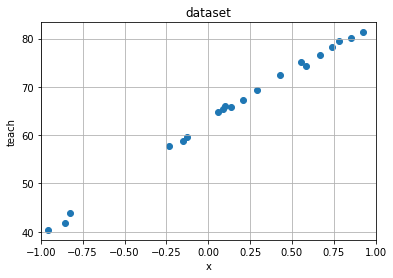
このノイズ付きモデルを用いてN回観測することで、N個の入出力ペア(\(input_i, output_i\))を得ることができる。これをデータセットとして利用する。これを実装したものが関数 make_dataset である。なお、観測結果のことを「関数の出力」という意味で出力と呼んでいるが、以下ではこれを教師データ(teach)と呼ぶことにする。
make_dataset で作成したデータセットがどのような分布になっているかを確認するため、 plot_rawdata により分布図として描画している。横軸が入力であり、縦軸が教師データである。
def true_function(x: np.ndarray) -> np.ndarray:
    """真のモデル
    本来は取得し得ない真のモデルを関数として表現したもの。
    Arguments:
        x (np.ndarray): サンプリング点の集合。
    Returns:
        np.ndarray: サンプリング点に対する真の値。
    """
    return 170 - 108 * np.exp(-0.2*x)

def make_dataset(num_of_samples: int, x_min: float, x_max: float,
                random_seed=0) -> Any:
    """真のモデルを用いてデータセットを作成。
    サンプリングの範囲は[x_min, x_max)。
    Arguments:
        num_of_samples (int): サンプル数。
        x_min, x_max (float): サンプリング範囲。
        random_seed (int): シード値。
    Returns:
        x (np.ndarray): サンプル点。
        teach (np.ndarray): サンプル点に対する観測値。true_funcionにノイズを付与。
    """
    np.random.seed(random_seed)
    x = np.random.rand(num_of_samples) * (x_max - x_min) + x_min
    noisy = np.random.rand(num_of_samples) * 2
    teach = true_function(x) + noisy
    return x, teach

num_of_samples = 20
x_min = -1.0
x_max = 1.0
x, teach = make_dataset(num_of_samples, x_min, x_max)
print(len(x), x)
print(len(teach), teach)
20 [ 0.09762701  0.43037873  0.20552675  0.08976637 -0.1526904   0.29178823
 -0.12482558  0.783546    0.92732552 -0.23311696  0.58345008  0.05778984
  0.13608912  0.85119328 -0.85792788 -0.8257414  -0.95956321  0.66523969
  0.5563135   0.7400243 ]
20 [66.04552636 72.50564637 67.2723329  65.48271027 58.88756061 69.40209033
 59.55653639 79.55445243 81.32617169 57.67476978 74.4241239  64.78954195
 65.81218245 80.04281038 41.82152035 43.84192567 40.37520695 76.68817051
 75.25949882 78.22153279]
def plot_rawdata(raw_x: np.ndarray, raw_teach: np.ndarray, x_min: float, x_max: float) -> None:
    """データセットを描画。
    Arguments:
        raw_x (np.ndarray): 入力値。
        raw_teach (np.ndarray): 観測値。
        x_min, x_max (float): 定義域(データセットのサンプリング範囲)。
    """
    plt.figure()
    plt.scatter(raw_x, raw_teach)
    plt.title("dataset")
    plt.xlabel("x")
    plt.ylabel("teach")
    plt.xlim(x_min, x_max)
    plt.grid(True)
    plt.show()
    #plt.savefig("rawdata.svg")

plot_rawdata(x, teach, x_min, x_max)
12.4. step 2: 線形回帰モデルによるMSE空間の観察。#
データセットは真の関数を知っていれば関数を介して入手することが可能だが、本来は知り得ず、何らかの方法で観測した結果N個の入出力ペア(\(input_i, teach_i\))しか手元には存在しない。このデータセットから、裏側にある真のモデルを予測しようとするのが機械学習だ。
データセットを表現するモデルとして線形回帰を採用しよう。線形回帰は1直線で入出力関係を表現するモデルであり、実データと予測結果との平均二乗誤差(MSE)が最小となるような直線により、事象を近似する。
関数 model は、線形回帰モデルを実装している。weight[0]は切片、weight[1]は傾きであり、入力inputを用いて算出することで予測結果を求めている。なお、切片や傾きのことをweight(重み)と書いているのは、モデルにとって「ある意味での重要度」を表現しているためだ。データセットに基づいて自動更新するパラメータという意味では parameter と書くことも多い。
関数 calc_mse は、モデルの良し悪しを判断するための指標としてMSEを求めるための関数だ。引数のinputは入力、teachは教師データであり、両方でデータセットを指定している。weightは線形回帰のための重みだ。データセットとweightが定まれば、その時のモデルがどのぐらい適切に事象を表現できているかを検証することができる。その指標の一つとしてMSEを求めている。
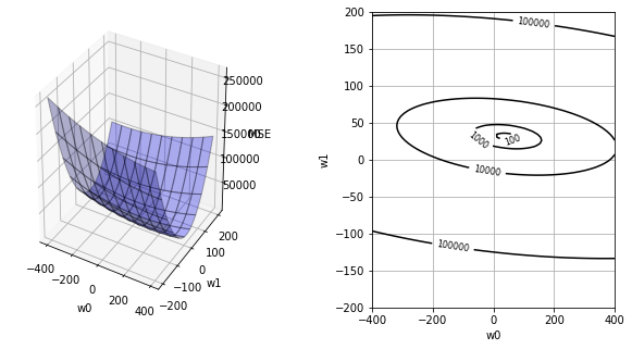
関数 plot_mse は、MSEに対する重みの影響を可視化している。具体的には、(1)で重みを手動で用意し、(2)でその時のMSEを算出、(3)全パターンのMSEを描画、という手順によりMSE空間を可視化している。これは「最適な重みとは何か」をイメージするために力技(無理やり)で描画しており、複雑な問題では容易ではないことを覚えておこう。
(1) モデルの切片weight[0]を-400〜+400、傾きweight[1]を-200〜+200までの範囲に限定し、各々を100分割した値を用意。
(2) 用意した重み毎にMSEを算出。
(3) 切片x傾きxMSEという3次元空間上に描画。
def model(input: np.ndarray, weights: List[Union[float, int]]) -> np.ndarray:
    """回帰モデルによる予測。
    Arguments:
        input (np.ndarray): モデルに対する入力。
        weights (list[number]): モデルの重み。
    Returns:
        predicted (np.ndarray): 入力に対する予測結果。
    """
    predicted = weights[0] + weights[1] * input
    return predicted

def calc_mse(input: np.ndarray, teach: np.ndarray, weights: List[Union[int, float]]):
    """MSE (Mean Squared Error) 算出。
    Arguments:
        input (np.ndarray): データセット(入力)。
        teach (np.ndarray): データセット(出力、観測値)。
        weights (list[number]): モデルの重み。
    Returns:
        mse (np.ndarray): MSE。
    """
    predicted = model(input, weights)
    mse = np.mean((predicted - teach)**2)
    return mse

def plot_mse(input: np.ndarray, teach: np.ndarray, weights_history=[None]):
    """重みに伴うMSE起伏の描画。
    Argumtns:
        input (np.ndarray): データセット(入力)。
        teach (np.ndarray): データセット(出力、観測値)。
        weights_history (np.ndarray): 勾配法による探索点移動のヒストリ。
    """
    dots = 100
    w0 = np.linspace(-400, 400, dots)
    w1 = np.linspace(-200, 200, dots)
    ww0, ww1 = np.meshgrid(w0, w1)
    MSE = np.zeros((len(w0), len(w1)))
    for i0 in range(dots):
        for i1 in range(dots):
            weights = [w0[i0], w1[i1]]
            MSE[i0, i1] = calc_mse(input, teach, weights)
    fig = plt.figure(figsize=(10, 5))
    plt.subplots_adjust(wspace=0.5)
    ax1 = fig.add_subplot(1, 2, 1, projection='3d')
    ax1.plot_surface(ww0, ww1, MSE, rstride=10, cstride=10, alpha=0.3, color='blue', edgecolor='black')
    ax1.set_xlabel("w0")
    ax1.set_ylabel("w1")
    ax1.set_zlabel("MSE")
    ax2 = fig.add_subplot(1, 2, 2)
    if len(weights_history) == 1:
        cont = ax2.contour(ww0, ww1, MSE, 30, colors='black', levels=[100, 1000, 10000, 100000])
        ax2.set_xlabel("w0")
        ax2.set_ylabel("w1")
        cont.clabel(fmt='%1.0f', fontsize=8)
        ax2.grid(True)
        #plt.show()
        plt.savefig('mse.svg')
    else:
        cont = ax2.contour(ww0, ww1, MSE, 30, colors='black', levels=[100, 1000, 10000, 100000])
        ax2.set_xlabel("w0")
        ax2.set_ylabel("w1")
        cont.clabel(fmt='%1.0f', fontsize=8)
        ax2.grid(True)
        ax2.scatter(weights_history[:,0], weights_history[:,1])
        plt.show()
        #plt.savefig('mse-history.svg')

plot_mse(x, teach)
12.5. step 3: 勾配法によるパラメータ探索の様子を確認。#
MSE空間を観察することが可能な小さい問題なら、可視化して最小MSEとなる重みを最適パラメータとすることができる。しかしながら一般的には可視化困難であり、何かしら別手段が必要となる。
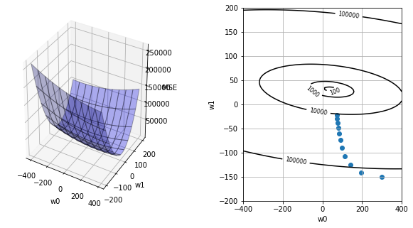
代表的なアルゴリズムとして勾配法を採用しよう。勾配法は、まずパラメータの初期値をランダムに設定する。次に、そこから得られる勾配情報をもとにより小さなMSEがあると見込まれるパラメータに移動する。この移動を繰り返して最適パラメータに辿り着こうとする。
関数 calc_slope は傾きを算出する関数である。
関数 gradient_descent は、勾配法を実装している。
出力結果は探索の様子を表している。history_id=0は、ランダムに設定した初期パラメータである。このときの傾き情報を元にパラメータを更新するという探索を9回目まで繰り返している。
def calc_slope(input: np.ndarray, teach: np.ndarray, weights: List[Union[int, float]]):
    """重み空間における傾きの算出。
    Argumtns:
        input (np.ndarray): データセット(入力)。
        teach (np.ndarray): データセット(出力、観測値)。
        weights (list[number]): モデルの重み。
    Returns:
        slope_w0, slope_w1 (float): 各変数に対する傾き。
    """
    predicted = model(input, weights)
    slope_w0 = np.mean(predicted - teach)
    slope_w1 = np.mean((predicted - teach) * input)
    return slope_w0, slope_w1

def gradient_descent(input: np.ndarray, teach: np.ndarray, alpha=0.5):
    """勾配法による適正重み探索。
    Arguments:
        input (np.ndarray): データセット(入力)。
        teach (np.ndarray): データセット(出力、観測値)。
        alpha (float > 0): 学習率(移動幅調整用パラメータ)。
    Returns:
        weights_history (np.ndarray): 探索した重みの履歴。
    """
    moving_max_count = 10
    weights_history = np.zeros((moving_max_count+1, 2))
    weights_history[0][0] = 300.
    weights_history[0][1] = -150.
    print("# begin gradin_descent")
    print("history_id, [w0, w1], (slope0, slope1)")
    for i in range(moving_max_count):
        slope = calc_slope(input, teach, weights_history[i])
        print(i, weights_history[i], slope)
        weights_history[i+1][0] = weights_history[i][0] - alpha * slope[0]
        weights_history[i+1][1] = weights_history[i][1] - alpha * slope[1]
    return weights_history

weights_history = gradient_descent(x, teach)
plot_mse(x, teach, weights_history)
# begin gradin_descent
history_id, [w0, w1], (slope0, slope1)
0 [ 300. -150.] (209.5843370987155, -18.219739876727658)
1 [ 195.20783145 -140.89013006] (106.27807623785165, -32.29587907509851)
2 [ 142.06879333 -124.74219052] (55.77292286969848, -35.61643748697637)
3 [ 114.1823319  -106.93397178] (30.791153744219667, -34.268302684684514)
4 [ 98.78675502 -89.79982044] (18.190322284246538, -31.105982356045622)
5 [ 89.69159388 -74.24682926] (11.632004074773572, -27.439559699578734)
6 [ 83.87559185 -60.52704941] (8.053830513663275, -23.845290405750553)
7 [ 79.84867659 -48.60440421] (5.971613731562999, -20.554273880259718)
8 [ 76.86286972 -38.32726727] (4.6621070652754835, -17.63830584600503)
9 [ 74.53181619 -29.50811434] (3.769542470784592, -15.098311214151176)
12.6. step 4: 探索により得たパラメータの良し悪しを確認。#
step 3 ではモデルの質をMSE空間により評価をしていたが、具体的な事象と比べてどのぐらい差があるのかを事象空間により確認してみよう。。
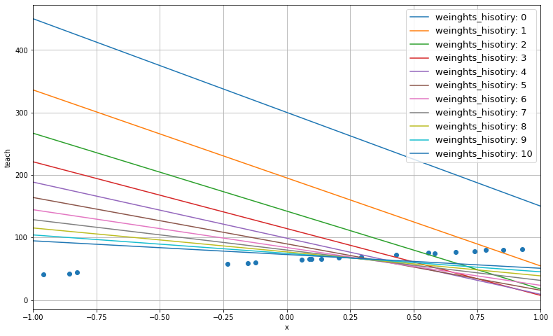
step 3では更新履歴0回目〜9回目までのパラメータを保存している。このときのパラメータを用いたモデルを事象空間で描画したのが plot_predictive_model である。
ランダムな値で用意された最初のモデル(id=0)は、データセットからとても大きく離れている。これが探索を繰り返す都度、少しずつデータセットの傾向に近づいている様子が観察できるだろう。
def plot_predictive_model(input, teach, x_min, x_max, weights_history):
    """重み履歴を用いた予測モデルの描画。
    Arguments:
        input (np.ndarray): データセット(入力)。
        teach (np.ndarray): データセット(出力、観測値)。
        x_min, x_max (float): データセット範囲。
        weights_history (np.ndarray): 探索した重みの履歴。
    """
    base = np.linspace(x_min, x_max, 100)
    predicted = []
    for i in range(len(weights_history)):
        w0 = weights_history[i][0]
        w1 = weights_history[i][1]
        predicted.append(w0 + w1 * base)
    plt.figure(figsize=(13,8))
    for i in range(len(weights_history)):
        line, = plt.plot(base, predicted[i])
        line.set_label('weinghts_hisotiry: {}'.format(i))
    plt.scatter(input, teach)
    plt.xlabel("x")
    plt.ylabel("teach")
    plt.xlim(x_min, x_max)
    plt.grid(True)
    plt.legend(loc='upper right', fontsize=13)
    plt.savefig('predicted_mode.svg')

plot_predictive_model(x, teach, x_min, x_max, weights_history)
12.7. others: 手動でパラメータ探してみよう#
演習説明
線形回帰モデルに必要なパラメータは傾きと切片の2つだ。下記コードではこれらのパラメータを任意に編集すると、その時の予測結果、教師データ、MSEを出力することができる。
演習内容
演習1: 手動でパラメータを変更し、小さなMSEとなる最適モデルを探してみよう。
演習2: データセットの散布図を描こう。(コードを書く必要があります)
演習3: 演習2の散布図に、獲得したモデルを描画しよう。(コードを書く必要があります)
# ランダムな値でパラメータ(傾きと切片)を用意してみよう。
切片 = 1.5
傾き = 50.0

parameters = np.array([切片, 傾き])

# 用意したパラメータの予測結果とMSEを求めてみよう。
予測結果 = model(x, parameters)
MSE = calc_mse(x, teach, parameters)
print("予測結果 = ", 予測結果)
print("教師データ = ", teach)
print("MSE = ", MSE)
予測結果 =  [  6.38135039  23.01893664  11.77633761   5.9883183   -6.13452007
  16.08941131  -4.74127887  40.67730008  47.86627605 -10.15584812
  30.67250381   4.38949198   8.30445611  44.05966383 -41.39639418
 -39.78707003 -46.47816026  34.76198455  29.31567509  38.50121482]
教師データ =  [66.04552636 72.50564637 67.2723329  65.48271027 58.88756061 69.40209033
 59.55653639 79.55445243 81.32617169 57.67476978 74.4241239  64.78954195
 65.81218245 80.04281038 41.82152035 43.84192567 40.37520695 76.68817051
 75.25949882 78.22153279]
MSE =  3406.8812794875325