
2. Example for Linear Regression
story (Procedure of applied ML)
Preparation
Make the purpose (goal) clear.
Make the task concrete.
Check the possibilities to replace the existing services.
Prepare the dataset
Select a model
Continue learning, evaluation and tuning
ref.
# Prepare the dataset
# Load the diabetes dataset
# ref. https://scikit-learn.org/stable/datasets/index.html#diabetes-dataset

from sklearn import datasets
diabetes = datasets.load_diabetes()

orig_X = diabetes.data # get a feature matrix (input dataset)
print(type(orig_X))    # check the type
print(orig_X.shape)    # check the size of feature matrix
print(orig_X[:5])      # display the first 5 samples
print(diabetes.feature_names)    # display the name of each element of feature
<class 'numpy.ndarray'>
(442, 10)
[[ 0.03807591  0.05068012  0.06169621  0.02187235 -0.0442235  -0.03482076
  -0.04340085 -0.00259226  0.01990842 -0.01764613]
 [-0.00188202 -0.04464164 -0.05147406 -0.02632783 -0.00844872 -0.01916334
   0.07441156 -0.03949338 -0.06832974 -0.09220405]
 [ 0.08529891  0.05068012  0.04445121 -0.00567061 -0.04559945 -0.03419447
  -0.03235593 -0.00259226  0.00286377 -0.02593034]
 [-0.08906294 -0.04464164 -0.01159501 -0.03665645  0.01219057  0.02499059
  -0.03603757  0.03430886  0.02269202 -0.00936191]
 [ 0.00538306 -0.04464164 -0.03638469  0.02187235  0.00393485  0.01559614
   0.00814208 -0.00259226 -0.03199144 -0.04664087]]
['age', 'sex', 'bmi', 'bp', 's1', 's2', 's3', 's4', 's5', 's6']
# Here, use just one feature 'bmi' for simple exercise
import numpy as np
X = diabetes.data[:, np.newaxis, 2]
print(X.shape)
print(X[:5])
(442, 1)
[[ 0.06169621]
 [-0.05147406]
 [ 0.04445121]
 [-0.01159501]
 [-0.03638469]]
y = diabetes.target
print(y.shape)
print(y[:5])
(442,)
[151.  75. 141. 206. 135.]
# split the dataset into training and testing set
num_of_training = 400

X_train = X[:num_of_training]
X_test = X[num_of_training:]

y_train = y[:num_of_training]
y_test = y[num_of_training:]

print(X_train.shape)
print(X_test.shape)
print(y_train.shape)
print(y_test.shape)
(400, 1)
(42, 1)
(400,)
(42,)
# Select a model
# => Linear Regression

from sklearn import linear_model

# Create linear regression object
regr = linear_model.LinearRegression()

# Train the model using the training set
regr.fit(X_train, y_train)

# Make predictions using the testing set
predicted = regr.predict(X_test)

# Check the predictions vs true answer
print(np.c_[predicted, y_test])
[[196.51241167 175.        ]
 [109.98667708  93.        ]
 [121.31742804 168.        ]
 [245.95568858 275.        ]
 [204.75295782 293.        ]
 [270.67732703 281.        ]
 [ 75.99442421  72.        ]
 [241.8354155  140.        ]
 [104.83633574 189.        ]
 [141.91879342 181.        ]
 [126.46776938 209.        ]
 [208.8732309  136.        ]
 [234.62493762 261.        ]
 [152.21947611 113.        ]
 [159.42995399 131.        ]
 [161.49009053 174.        ]
 [229.47459628 257.        ]
 [221.23405012  55.        ]
 [129.55797419  84.        ]
 [100.71606266  42.        ]
 [118.22722323 146.        ]
 [168.70056841 212.        ]
 [227.41445974 233.        ]
 [115.13701842  91.        ]
 [163.55022706 111.        ]
 [114.10695016 152.        ]
 [120.28735977 120.        ]
 [158.39988572  67.        ]
 [237.71514243 310.        ]
 [121.31742804  94.        ]
 [ 98.65592612 183.        ]
 [123.37756458  66.        ]
 [205.78302609 173.        ]
 [ 95.56572131  72.        ]
 [154.27961264  49.        ]
 [130.58804246  64.        ]
 [ 82.17483382  48.        ]
 [171.79077322 178.        ]
 [137.79852034 104.        ]
 [137.79852034 132.        ]
 [190.33200206 220.        ]
 [ 83.20490209  57.        ]]
# Check the differences (errors)
print(y_test - predicted)
[ -21.51241167  -16.98667708   46.68257196   29.04431142   88.24704218
   10.32267297   -3.99442421 -101.8354155    84.16366426   39.08120658
   82.53223062  -72.8732309    26.37506238  -39.21947611  -28.42995399
   12.50990947   27.52540372 -166.23405012  -45.55797419  -58.71606266
   27.77277677   43.29943159    5.58554026  -24.13701842  -52.55022706
   37.89304984   -0.28735977  -91.39988572   72.28485757  -27.31742804
   84.34407388  -57.37756458  -32.78302609  -23.56572131 -105.27961264
  -66.58804246  -34.17483382    6.20922678  -33.79852034   -5.79852034
   29.66799794  -26.20490209]
# Check the sum of absolute error
print(sum(np.abs(y_test - predicted)))

# MAE (Mean Absolute Error)
print(sum(np.abs(y_test - predicted)) / len(X_test))
1890.1633693291935
45.00388974593318
# Plot testing set and predictions
%matplotlib inline
import matplotlib.pyplot as plt
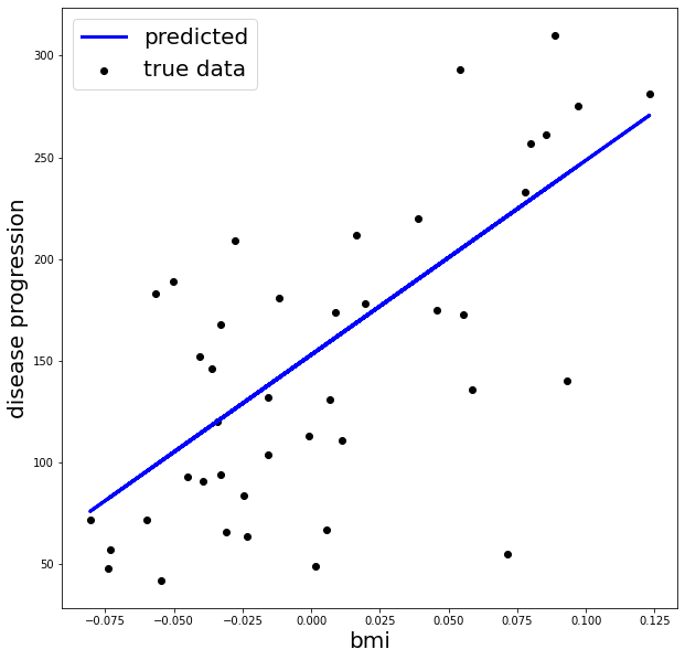
fig, ax = plt.subplots(1, 1, figsize=(10, 10))
ax.scatter(X_test, y_test, color='black', label='true data')
ax.plot(X_test, predicted, color='blue', linewidth=3, label='predicted')
ax.legend(loc='best', fontsize=20)
ax.set_xlabel('bmi', fontsize=20)
ax.set_ylabel('disease progression', fontsize=20)
plt.show()
# Check the model (obtained parameters)
print('coefficients: ', regr.coef_)
print('intercept: ', regr.intercept_)
coefficients:  [955.70303385]
intercept:  153.00018395675963