2. 数値データに対する前処理コード例¶

ref.
- preprocess methods
  - 機械学習のための特徴量エンジニアリング
  - 5.3. Preprocessing data
- data: YouTuberデータセット公開してみた
全体の流れ
- データセットの準備。
- 数値データに対する前処理の例
  - 手法1：バイナリ化
  - 手法2：アドホックな離散化
  - 手法3：統計的な離散化
  - 手法4：ログスケール化
    - デフォルトとログスケールとの比較
  - 手法5：標準化
  - 手法6：min-maxスケーリング
- 特徴ベクトルに対する前処理の例
  - 手法7：正規化
  - 手法8：正規分布への写像
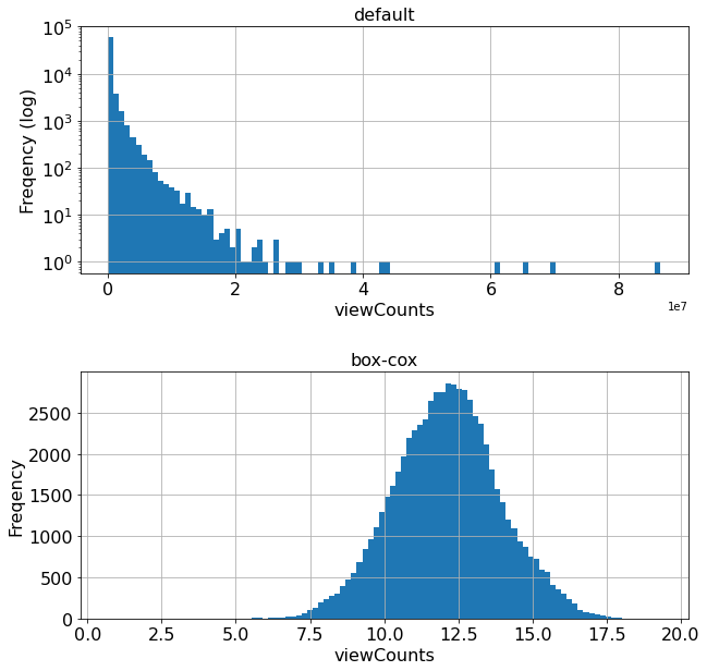
    - デフォルトとbox-cox写像との比較

2.1. 環境構築¶

!pip install quilt
!quilt install haradai1262/YouTuber

Collecting quilt
?25l  Downloading https://files.pythonhosted.org/packages/cf/17/5f30e1726fb8a311bb5b976f8deb37580f931d077ceeefb263424955ce4a/quilt-2.9.15-py3-none-any.whl (110kB)

     |███                             | 10kB 14.7MB/s eta 0:00:01
     |██████                          | 20kB 18.9MB/s eta 0:00:01
     |█████████                       | 30kB 22.0MB/s eta 0:00:01
     |███████████▉                    | 40kB 25.1MB/s eta 0:00:01
     |██████████████▉                 | 51kB 27.1MB/s eta 0:00:01
     |█████████████████▉              | 61kB 27.9MB/s eta 0:00:01
     |████████████████████▊           | 71kB 27.8MB/s eta 0:00:01
     |███████████████████████▊        | 81kB 29.0MB/s eta 0:00:01
     |██████████████████████████▊     | 92kB 30.1MB/s eta 0:00:01
     |█████████████████████████████▊  | 102kB 31.6MB/s eta 0:00:01
     |████████████████████████████████| 112kB 31.6MB/s 
?25hRequirement already satisfied: requests>=2.12.4 in /usr/local/lib/python3.7/dist-packages (from quilt) (2.23.0)
Requirement already satisfied: pyyaml>=3.12 in /usr/local/lib/python3.7/dist-packages (from quilt) (3.13)
Requirement already satisfied: numpy>=1.14.0 in /usr/local/lib/python3.7/dist-packages (from quilt) (1.19.5)
Requirement already satisfied: future>=0.16.0 in /usr/local/lib/python3.7/dist-packages (from quilt) (0.16.0)
Requirement already satisfied: pandas>=0.21.0 in /usr/local/lib/python3.7/dist-packages (from quilt) (1.1.5)
Requirement already satisfied: pyarrow>=0.9.0 in /usr/local/lib/python3.7/dist-packages (from quilt) (3.0.0)
Requirement already satisfied: tqdm>=4.11.2 in /usr/local/lib/python3.7/dist-packages (from quilt) (4.41.1)
Requirement already satisfied: packaging>=16.8 in /usr/local/lib/python3.7/dist-packages (from quilt) (20.9)
Requirement already satisfied: appdirs>=1.4.0 in /usr/local/lib/python3.7/dist-packages (from quilt) (1.4.4)
Requirement already satisfied: six>=1.10.0 in /usr/local/lib/python3.7/dist-packages (from quilt) (1.15.0)
Requirement already satisfied: xlrd>=1.0.0 in /usr/local/lib/python3.7/dist-packages (from quilt) (1.1.0)
Requirement already satisfied: idna<3,>=2.5 in /usr/local/lib/python3.7/dist-packages (from requests>=2.12.4->quilt) (2.10)
Requirement already satisfied: urllib3!=1.25.0,!=1.25.1,<1.26,>=1.21.1 in /usr/local/lib/python3.7/dist-packages (from requests>=2.12.4->quilt) (1.24.3)
Requirement already satisfied: certifi>=2017.4.17 in /usr/local/lib/python3.7/dist-packages (from requests>=2.12.4->quilt) (2020.12.5)
Requirement already satisfied: chardet<4,>=3.0.2 in /usr/local/lib/python3.7/dist-packages (from requests>=2.12.4->quilt) (3.0.4)
Requirement already satisfied: python-dateutil>=2.7.3 in /usr/local/lib/python3.7/dist-packages (from pandas>=0.21.0->quilt) (2.8.1)
Requirement already satisfied: pytz>=2017.2 in /usr/local/lib/python3.7/dist-packages (from pandas>=0.21.0->quilt) (2018.9)
Requirement already satisfied: pyparsing>=2.0.2 in /usr/local/lib/python3.7/dist-packages (from packaging>=16.8->quilt) (2.4.7)
Installing collected packages: quilt
Successfully installed quilt-2.9.15
Downloading package metadata...
Downloading 4 fragments (633095200 bytes before compression)...
100% 633M/633M [00:18<00:00, 34.4MB/s]

2.2. データセットの準備¶

from quilt.data.haradai1262 import YouTuber
import numpy as np
import pandas as pd
import matplotlib.pyplot as plt

#df = YouTuber.channels.UUUM()
df = YouTuber.channel_videos.UUUM_videos()

# check the descriptive statistics of numerical data
df.describe()

	viewCount	likeCount	favoriteCount	dislikeCount	commentCount	TopicIds	idx
count	6.627900e+04	64256.000000	66289.0	64256.000000	65997.000000	0.0	66289.000000
mean	4.545539e+05	3233.703390	0.0	296.430014	533.418807	NaN	235.730136
std	1.328105e+06	9768.090605	0.0	1633.734833	2253.437482	NaN	142.868881
min	0.000000e+00	0.000000	0.0	0.000000	0.000000	NaN	1.000000
25%	3.907100e+04	266.000000	0.0	23.000000	55.000000	NaN	111.000000
50%	1.214190e+05	776.000000	0.0	67.000000	150.000000	NaN	229.000000
75%	3.512260e+05	2260.000000	0.0	201.000000	394.000000	NaN	357.000000
max	8.664236e+07	630051.000000	0.0	213677.000000	227598.000000	NaN	501.000000

# the description of data frame
df.head()

	id	title	description	liveBroadcastContent	tags	publishedAt	thumbnails	viewCount	likeCount	dislikeCount	commentCount	caption	definition	dimension	duration	projection	TopicIds	relevantTopicIds	idx	cid
0	R7V5d94XkGQ	【大食い】超高級寿司店で３人で食べ放題したらいくらかかるの!?【大トロ1カン2,000円】	提供：ポコロンダンジョンズ\r\r\r\r\niOS：https://bit.ly/2sGg...	none	['ヒカキン', 'ヒカキンtv', 'hikakintv', 'hikakin', 'ひか...	2018-06-30T04:00:01.000Z	https://i.ytimg.com/vi/R7V5d94XkGQ/default.jpg	2244205.0	27703.0	3667.0	8647.0	False	hd	2d	PT21M16S	rectangular	NaN	['/m/02wbm', '/m/019_rr', '/m/019_rr', '/m/02w...	1	UCZf__ehlCEBPop___sldpBUQ
1	2R9_bkcWNd4	【女王集結】女性YouTuberたちと飲みながら本音トークしてみたら爆笑www	しばなんチャンネルの動画\r\r\r\r\nhttps://www.youtube.com/...	none	['ヒカキン', 'ヒカキンtv', 'hikakintv', 'hikakin', 'ひか...	2018-06-29T08:00:01.000Z	https://i.ytimg.com/vi/2R9_bkcWNd4/default.jpg	1869268.0	30889.0	3483.0	8859.0	False	hd	2d	PT18M38S	rectangular	NaN	['/m/04rlf', '/m/02jjt', '/m/02jjt']	2	UCZf__ehlCEBPop___sldpBUQ
2	EU8S-zxS9PI	【悪質】偽物ヒカキン許さねぇ…注意してください！【なりすまし】	◆チャンネル登録はこちら↓\r\r\r\r\nhttp://www.youtube.com/...	none	['ヒカキン', 'ヒカキンtv', 'hikakintv', 'hikakin', 'ひか...	2018-06-27T08:38:55.000Z	https://i.ytimg.com/vi/EU8S-zxS9PI/default.jpg	1724625.0	33038.0	4298.0	11504.0	False	hd	2d	PT6M12S	rectangular	NaN	['/m/04rlf', '/m/02jjt', '/m/02jjt']	3	UCZf__ehlCEBPop___sldpBUQ
3	5wnfkIfw0jE	ツイッターのヒカキンシンメトリーBotが面白すぎて爆笑www	◆チャンネル登録はこちら↓\r\r\r\r\nhttp://www.youtube.com/...	none	['ヒカキン', 'ヒカキンtv', 'hikakintv', 'hikakin', 'ひか...	2018-06-25T07:46:07.000Z	https://i.ytimg.com/vi/5wnfkIfw0jE/default.jpg	1109029.0	25986.0	5063.0	6852.0	False	hd	2d	PT6M31S	rectangular	NaN	['/m/04rlf', '/m/02jjt', '/m/02jjt']	4	UCZf__ehlCEBPop___sldpBUQ
4	-6duBsde_XM	【放送事故】酒飲みながら東海オンエア×ヒカキンで質問コーナーやったらヤバかったwww	提供：モンスターストライク\r\r\r\r\n▼キャンペーンサイトはこちら\r\r\r\r\...	none	['ヒカキン', 'ヒカキンtv', 'hikakintv', 'hikakin', 'ひか...	2018-06-21T08:00:00.000Z	https://i.ytimg.com/vi/-6duBsde_XM/default.jpg	1759797.0	33923.0	2150.0	4517.0	False	hd	2d	PT27M7S	rectangular	NaN	['/m/098wr', '/m/019_rr', '/m/02wbm', '/m/019_...	5	UCZf__ehlCEBPop___sldpBUQ

# column 'viewCount''
df['viewCount'].sort_values()

  0.0
  0.0
  0.0
  0.0
  0.0
        ... 
  NaN
  NaN
  NaN
  NaN
  NaN
Name: viewCount, Length: 66289, dtype: float64

# drop samples including NaN & 0 on 'viewCount'

print('orig_num = ', len(df))
print('num of NaN = ', len(df.query('viewCount == "NaN"')))
df = df[df['viewCount'].notnull()]
print('after_num = ', len(df))

df = df[df['viewCount'] != 0]
print('after_num2 = ', len(df))

orig_num =  66289
num of NaN =  10
after_num =  66279
after_num2 =  66231

df['viewCount'].describe()

count    6.623100e+04
mean     4.548834e+05
std      1.328530e+06
min      2.000000e+00
25%      3.919150e+04
50%      1.215850e+05
75%      3.515195e+05
max      8.664236e+07
Name: viewCount, dtype: float64

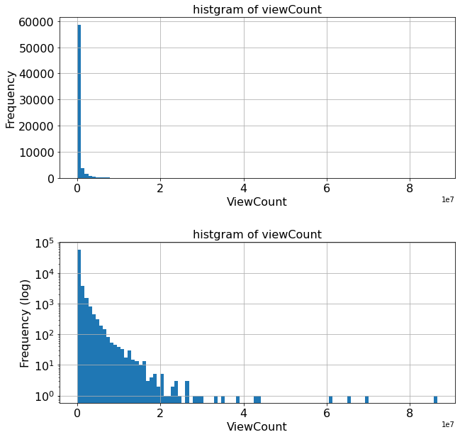
# histgram of viewCount

%matplotlib inline
fontsize = 16

fig, (ax1, ax2) = plt.subplots(2, 1, figsize=(10,10))
fig.subplots_adjust(hspace=0.4)

# default values
df['viewCount'].hist(ax=ax1, bins=100)
ax1.tick_params(labelsize=fontsize)
ax1.set_title('histgram of viewCount', fontsize=fontsize)
ax1.set_xlabel('ViewCount', fontsize=fontsize)
ax1.set_ylabel('Frequency', fontsize=fontsize)

# log
df['viewCount'].hist(ax=ax2, bins=100, log=True)
ax2.tick_params(labelsize=fontsize)
ax2.set_title('histgram of viewCount', fontsize=fontsize)
ax2.set_xlabel('ViewCount', fontsize=fontsize)
ax2.set_ylabel('Frequency (log)', fontsize=fontsize)

Text(0, 0.5, 'Frequency (log)')

2.3. 数値データに対する前処理の例¶

2.3.1. 手法1：バイナリ化(binarization)¶

# preprocess method 1: binarization by mean value

THRESHOLD = df['viewCount'].mean()
new_column = df['viewCount'] > THRESHOLD
new_column = np.where(new_column == True, 1, 0)
temp = pd.DataFrame(df['viewCount'])
temp['binary'] = new_column
temp.head()

	viewCount	binary
0	2244205.0	1
1	1869268.0	1
2	1724625.0	1
3	1109029.0	1
4	1759797.0	1

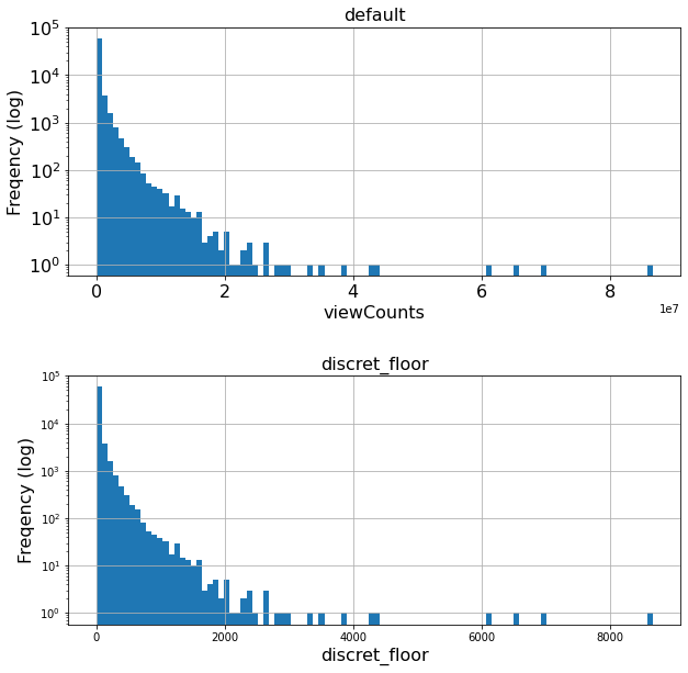
2.3.2. 手法2：アドホックな離散化(ad-hoc discretization)¶

# preprocess method 2: discretization 1, ad-hoc division
floor = 10000
new_column = np.floor_divide(df['viewCount'], floor)
temp['discret_floor'] = new_column
temp.head()

	viewCount	binary	discret_floor
0	2244205.0	1	224.0
1	1869268.0	1	186.0
2	1724625.0	1	172.0
3	1109029.0	1	110.0
4	1759797.0	1	175.0

fig, (ax1, ax2) = plt.subplots(2, 1, figsize=(10,10))
fig.subplots_adjust(hspace=0.4)

# default values
temp['viewCount'].hist(ax=ax1, bins=100, log=True)
ax1.tick_params(labelsize=fontsize)
ax1.set_title('default', fontsize=fontsize)
ax1.set_xlabel('viewCounts', fontsize=fontsize)
ax1.set_ylabel('Freqency (log)', fontsize=fontsize)

# discret_floor
temp['discret_floor'].hist(ax=ax2, bins=100, log=True)
ax2.set_title('discret_floor', fontsize=fontsize)
ax2.set_xlabel('discret_floor', fontsize=fontsize)
ax2.set_ylabel('Freqency (log)', fontsize=fontsize)

Text(0, 0.5, 'Freqency (log)')

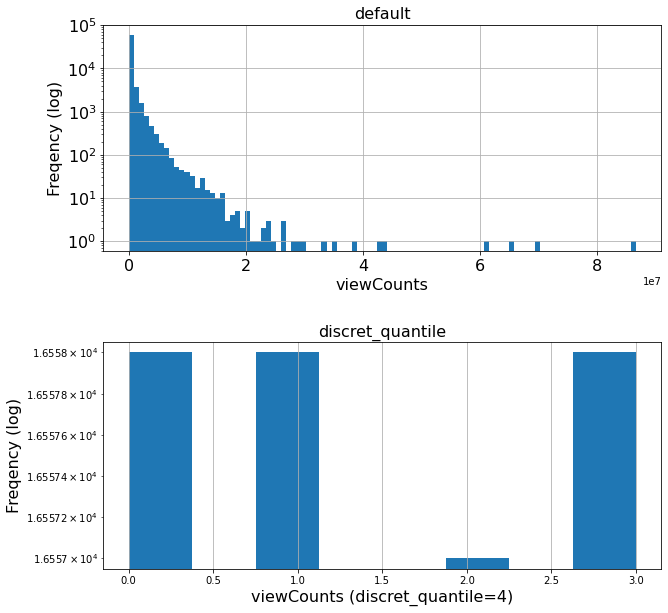
../_images/preprocess_numerical_15_1.png

2.3.3. 手法3：統計的な離散化¶

# preprocess method 3: discretization 2, quantilzation
discret_num = 4
ranges = np.linspace(0, 1, discret_num)
data = df['viewCount'].quantile(ranges)
data

000000    2.000000e+00
333333    5.913133e+04
666667    2.408843e+05
000000    8.664236e+07
Name: viewCount, dtype: float64

new_column = pd.qcut(df['viewCount'], discret_num, labels=False)
temp['discret_quantile'] = new_column
temp

	viewCount	binary	discret_floor	discret_quantile
0	2244205.0	1	224.0	3
1	1869268.0	1	186.0	3
2	1724625.0	1	172.0	3
3	1109029.0	1	110.0	3
4	1759797.0	1	175.0	3
...	...	...	...	...
66284	131489.0	0	13.0	2
66285	13271.0	0	1.0	0
66286	76266.0	0	7.0	1
66287	282447.0	0	28.0	2
66288	6900.0	0	0.0	0

66231 rows × 4 columns

fig, (ax1, ax2) = plt.subplots(2, 1, figsize=(10,10))
fig.subplots_adjust(hspace=0.4)

# default values
temp['viewCount'].hist(ax=ax1, bins=100, log=True)
ax1.tick_params(labelsize=fontsize)
ax1.set_title('default', fontsize=fontsize)
ax1.set_xlabel('viewCounts', fontsize=fontsize)
ax1.set_ylabel('Freqency (log)', fontsize=fontsize)

# discret_quantile
bins = discret_num*2
temp['discret_quantile'].hist(ax=ax2, bins=bins, log=True)
ax2.set_title('discret_quantile', fontsize=fontsize)
ax2.set_xlabel('viewCounts (discret_quantile={})'.format(discret_num), fontsize=fontsize)
ax2.set_ylabel('Freqency (log)', fontsize=fontsize)

Text(0, 0.5, 'Freqency (log)')

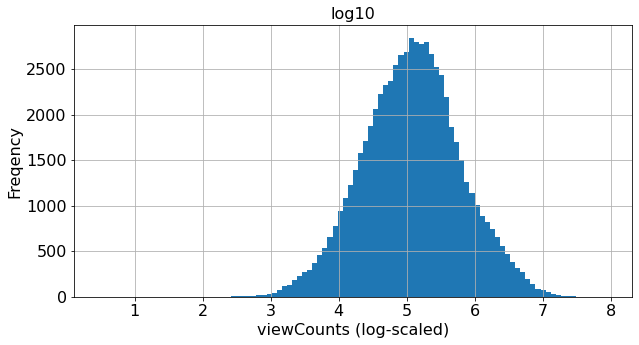
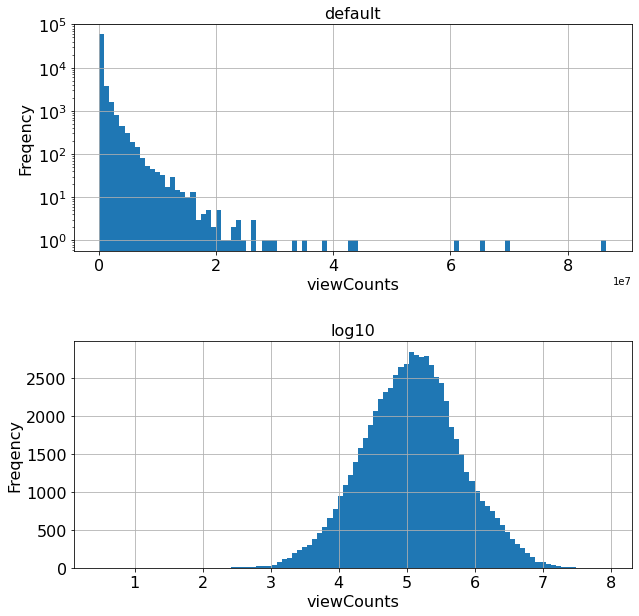
../_images/preprocess_numerical_19_1.png

2.3.4. 手法4：ログスケール化(log-scaling)¶

# preprocess method 4: log-scaling
new_column = np.log10(df['viewCount'] + 1)
temp['log10'] = new_column
temp.head()

	viewCount	binary	discret_floor	discret_quantile	log10
0	2244205.0	1	224.0	3	6.351063
1	1869268.0	1	186.0	3	6.271672
2	1724625.0	1	172.0	3	6.236695
3	1109029.0	1	110.0	3	6.044943
4	1759797.0	1	175.0	3	6.245463

2.3.5. デフォルトとログスケールとの比較¶

fig, (ax1, ax2) = plt.subplots(2, 1, figsize=(10,10))
fig.subplots_adjust(hspace=0.4)

# default values
temp['viewCount'].hist(ax=ax1, bins=100, log=True)
ax1.tick_params(labelsize=fontsize)
ax1.set_title('default', fontsize=fontsize)
ax1.set_xlabel('viewCounts', fontsize=fontsize)
ax1.set_ylabel('Freqency', fontsize=fontsize)

# log-scaled
temp['log10'].hist(ax=ax2, bins=100)
ax2.tick_params(labelsize=fontsize)
ax2.set_title('log10', fontsize=fontsize)
ax2.set_xlabel('viewCounts', fontsize=fontsize)
ax2.set_ylabel('Freqency', fontsize=fontsize)

Text(0, 0.5, 'Freqency')

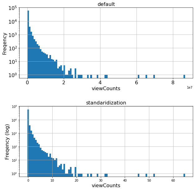
../_images/preprocess_numerical_23_1.png

2.3.6. 手法5：標準化(standardization)¶

from sklearn import preprocessing

data = np.array(df['viewCount'].values, dtype='float64')
data = data.reshape(len(data), 1)
new_column = preprocessing.scale(data)
temp['standardization'] = new_column
temp.head()

	viewCount	binary	discret_floor	discret_quantile	log10	standardization
0	2244205.0	1	224.0	3	6.351063	1.346854
1	1869268.0	1	186.0	3	6.271672	1.064632
2	1724625.0	1	172.0	3	6.236695	0.955757
3	1109029.0	1	110.0	3	6.044943	0.492387
4	1759797.0	1	175.0	3	6.245463	0.982231

mean = np.mean(new_column)
var = np.var(new_column)
print('mean = ', mean, ', var = ', var)

temp['standardization'].describe()

mean =  1.2873900181367037e-17 , var =  1.0

count    6.623100e+04
mean     8.899653e-16
std      1.000008e+00
min     -3.423971e-01
25%     -3.128985e-01
50%     -2.508795e-01
75%     -7.780379e-02
max      6.487481e+01
Name: standardization, dtype: float64

fig, (ax1, ax2) = plt.subplots(2, 1, figsize=(10,10))
fig.subplots_adjust(hspace=0.4)

# default values
temp['viewCount'].hist(ax=ax1, bins=100, log=True)
ax1.tick_params(labelsize=fontsize)
ax1.set_title('default', fontsize=fontsize)
ax1.set_xlabel('viewCounts', fontsize=fontsize)
ax1.set_ylabel('Freqency', fontsize=fontsize)

# log-scaled
ax2.set_title('standaridization', fontsize=fontsize)
ax2.set_xlabel('viewCounts', fontsize=fontsize)
ax2.set_ylabel('Freqency (log)', fontsize=fontsize)
temp['standardization'].hist(ax=ax2, bins=100, log=True)
#plt.hist(temp['standardization'], bins=100, log=True)

<matplotlib.axes._subplots.AxesSubplot at 0x7fa9057fc550>

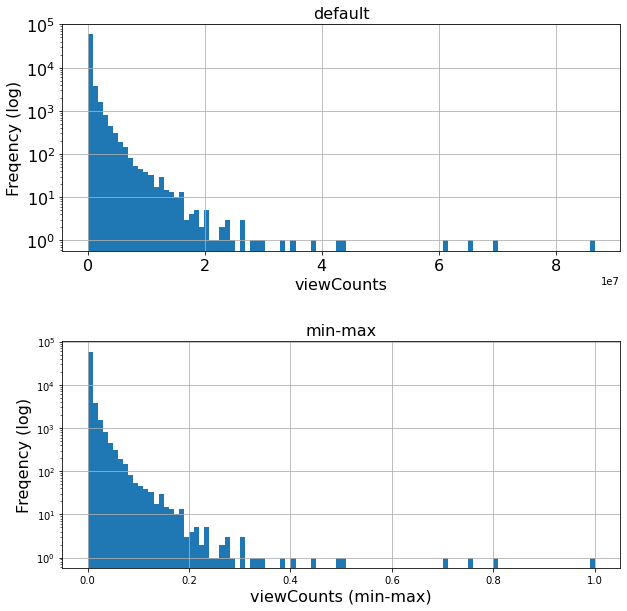
../_images/preprocess_numerical_27_1.png

2.3.7. 手法6：min-maxスケーリング(Min-Max scalering)¶

min-max scaler

"""
min = data.min(axis=0)
max = data.max(axis=0)
new_column = (data - min) / (max - min)
temp['min-max'] = new_column
temp.head()
"""

new_column = preprocessing.minmax_scale(df['viewCount'])
temp['min-max'] = new_column
temp.head()

	viewCount	binary	discret_floor	discret_quantile	log10	standardization	min-max
0	2244205.0	1	224.0	3	6.351063	1.346854	0.025902
1	1869268.0	1	186.0	3	6.271672	1.064632	0.021575
2	1724625.0	1	172.0	3	6.236695	0.955757	0.019905
3	1109029.0	1	110.0	3	6.044943	0.492387	0.012800
4	1759797.0	1	175.0	3	6.245463	0.982231	0.020311

fig, (ax1, ax2) = plt.subplots(2, 1, figsize=(10,10))
fig.subplots_adjust(hspace=0.4)

# default values
temp['viewCount'].hist(ax=ax1, bins=100, log=True)
ax1.tick_params(labelsize=fontsize)
ax1.set_title('default', fontsize=fontsize)
ax1.set_xlabel('viewCounts', fontsize=fontsize)
ax1.set_ylabel('Freqency (log)', fontsize=fontsize)

# min-max
ax2.set_title('min-max', fontsize=fontsize)
ax2.set_xlabel('viewCounts (min-max)', fontsize=fontsize)
ax2.set_ylabel('Freqency (log)', fontsize=fontsize)
temp['min-max'].hist(ax=ax2, bins=100, log=True)

<matplotlib.axes._subplots.AxesSubplot at 0x7fa905211f10>

../_images/preprocess_numerical_30_1.png

2.4. 特徴ベクトルに対する前処理の例¶

2.4.1. 手法7：正規化(normalization)¶

正規化という考え方自体は特徴量（データセットを表と見た時の列）に対しても適用できる。ここでは特徴ベクトル（行）に対して適用した際の値を観察する。
NOTE: the process target is NOT one feature value (one column). The target of normalization is “feature vector (one row)”.
5.3.3. Normalization

temp.head()

	viewCount	binary	discret_floor	discret_quantile	log10	standardization	min-max
0	2244205.0	1	224.0	3	6.351063	1.346854	0.025902
1	1869268.0	1	186.0	3	6.271672	1.064632	0.021575
2	1724625.0	1	172.0	3	6.236695	0.955757	0.019905
3	1109029.0	1	110.0	3	6.044943	0.492387	0.012800
4	1759797.0	1	175.0	3	6.245463	0.982231	0.020311

normalized_l2 = preprocessing.normalize(temp, norm='l2')
normalized_l2 = pd.DataFrame(normalized_l2, columns=temp.columns)
normalized_l2.head()

	viewCount	binary	discret_floor	discret_quantile	log10	standardization	min-max
0	1.0	4.455921e-07	0.000100	0.000001	0.000003	6.001473e-07	1.154169e-08
1	1.0	5.349688e-07	0.000100	0.000002	0.000003	5.695449e-07	1.154169e-08
2	1.0	5.798362e-07	0.000100	0.000002	0.000004	5.541823e-07	1.154169e-08
3	1.0	9.016897e-07	0.000099	0.000003	0.000005	4.439801e-07	1.154168e-08
4	1.0	5.682474e-07	0.000099	0.000002	0.000004	5.581503e-07	1.154169e-08

sum = 0
for item in normalized_l2.values[0]:
    sum += item ** 2
print('L2 norm = ', sum)

L2 norm =  0.9999999999999999

2.4.2. 手法8：正規分布への写像(Mapping to a Gaussian distribution)¶

Mapping to a Gaussian distribution

pt = preprocessing.PowerTransformer(method='box-cox', standardize=False)
orig = df['viewCount'].values.reshape(-1,1)
new_column = pt.fit_transform(orig)
temp['box-cox'] = new_column
temp.head()

	viewCount	binary	discret_floor	discret_quantile	log10	standardization	min-max	box-cox
0	2244205.0	1	224.0	3	6.351063	1.346854	0.025902	15.286494
1	1869268.0	1	186.0	3	6.271672	1.064632	0.021575	15.086987
2	1724625.0	1	172.0	3	6.236695	0.955757	0.019905	14.999160
3	1109029.0	1	110.0	3	6.044943	0.492387	0.012800	14.518429
4	1759797.0	1	175.0	3	6.245463	0.982231	0.020311	15.021172

2.4.3. デフォルトとBox-Cox写像との比較¶

fig, (ax1, ax2) = plt.subplots(2, 1, figsize=(10,10))
fig.subplots_adjust(hspace=0.4)

# default values
temp['viewCount'].hist(ax=ax1, bins=100, log=True)
ax1.tick_params(labelsize=fontsize)
ax1.set_title('default', fontsize=fontsize)
ax1.set_xlabel('viewCounts', fontsize=fontsize)
ax1.set_ylabel('Freqency (log)', fontsize=fontsize)

# box-cox
temp['box-cox'].hist(ax=ax2, bins=100)
ax2.tick_params(labelsize=fontsize)
ax2.set_title('box-cox', fontsize=fontsize)
ax2.set_xlabel('viewCounts', fontsize=fontsize)
ax2.set_ylabel('Freqency', fontsize=fontsize)

Text(0, 0.5, 'Freqency')

../_images/preprocess_numerical_39_1.png

# 似ている分布、log-scaledとの比較

fig, ax = plt.subplots(figsize=(10,5))

# log-scaled
temp['log10'].hist(ax=ax, bins=100)
ax.tick_params(labelsize=fontsize)
ax.set_title('log10', fontsize=fontsize)
ax.set_xlabel('viewCounts (log-scaled)', fontsize=fontsize)
ax.set_ylabel('Freqency', fontsize=fontsize)

Text(0, 0.5, 'Freqency')

../_images/preprocess_numerical_40_1.png

データマイニング

2. 数値データに対する前処理コード例¶

2.1. 環境構築¶

2.2. データセットの準備¶

2.3. 数値データに対する前処理の例¶

2.3.1. 手法1：バイナリ化(binarization)¶

2.3.2. 手法2：アドホックな離散化(ad-hoc discretization)¶

2.3.3. 手法3：統計的な離散化¶

2.3.4. 手法4：ログスケール化(log-scaling)¶

2.3.5. デフォルトとログスケールとの比較¶

2.3.6. 手法5：標準化(standardization)¶

2.3.7. 手法6：min-maxスケーリング(Min-Max scalering)¶

2.4. 特徴ベクトルに対する前処理の例¶

2.4.1. 手法7：正規化(normalization)¶

2.4.2. 手法8：正規分布への写像(Mapping to a Gaussian distribution)¶

2.4.3. デフォルトとBox-Cox写像との比較¶